scikit-learnのランダムフォレスト回帰手を動かして学ぶ

scikit-learnデータ分析実装ハンドブックのサンプルコードを実際にコードを動かす

ひととり読み終えたのだが、やはり実際にコードを動かさないとイメージが沸かない。jupyter lab(Jupyter Notebookの後継) で実際に動かしたことを記録しておく。やや古い本(と言っても、2019年末初版の本なのでそこまで古くないのだけどこの界隈は今発展速度が速すぎるので)だから、一部書籍公開サンプルコードが動作しない箇所があるので、それの訂正ものせておきます。

jupyter labでの動作結果

# ライブラリのインポート
%matplotlib inline
import matplotlib.pyplot as plt
import numpy as np
import pandas as pd
from sklearn.ensemble import RandomForestRegressor
from sklearn.model_selection import train_test_split
from sklearn.metrics import mean_squared_error
from sklearn.datasets import load_boston

%matplotlib inline
は、jupyter lab独特の記述
アウトプット行内（in line）にグラフが出力されるようにする。
ポップアップでは無く、アウトプット行にグラフを表示できるから便利

# 住宅価格データセットのダウンロード
# boston = load_boston()
# X = boston.data
# y = boston.target

data_url = "http://lib.stat.cmu.edu/datasets/boston"
raw_df = pd.read_csv(data_url, sep="\s+", skiprows=22, header=None)
x = np.hstack([raw_df.values[::2, :], raw_df.values[1::2, :2]])
y = raw_df.values[1::2, 2]

# 特徴量と正解を訓練データとテストデータに分割
X_train, X_test, y_train, y_test = train_test_split(X, y, test_size=0.2, random_state=0)
print('X_trainの形状：',X_train.shape,' y_trainの形状：',y_train.shape,' X_testの形状：',X_test.shape,' y_testの形状：',y_test.shape)

boston = load_boston()
という記載は、2022/12現在利用できない。倫理的な問題で利用は推奨していないとのこと。（犯罪率や黒人の割合などが含まれている為とのこと）
あくまで、機械学習のお勉強に利用する為、代替表記をしている

X_trainの形状： (404, 13)  y_trainの形状： (404,)  X_testの形状： (102, 13)  y_testの形状： (102,)

# ランダムフォレスト回帰のモデルを作成
# model = RandomForestRegressor(bootstrap=True, n_estimators=1000, criterion='mse', max_depth=None, random_state=0, n_jobs=-1)
model = RandomForestRegressor(bootstrap=True, n_estimators=1000, criterion='squared_error', max_depth=None, random_state=0, n_jobs=-1)

# モデルの訓練
model.fit(X_train, y_train)

criterion='mse'は、非推奨になっていて警告が派生するので、 criterion='squared_error' に書き換えている。

RandomForestRegressor(n_estimators=1000, n_jobs=-1, random_state=0)

In a Jupyter environment, please rerun this cell to show the HTML representation or trust the notebook.
On GitHub, the HTML representation is unable to render, please try loading this page with nbviewer.org.RandomForestRegressor

RandomForestRegressor(n_estimators=1000, n_jobs=-1, random_state=0)

# 訓練データ、テストデータの住宅価格を予測
y_train_pred = model.predict(X_train)
y_test_pred = model.predict(X_test)

# 正解の住宅価格と予測の住宅価格のMSEを計算
print('MSE train: %.2f, test: %.2f' % (
        mean_squared_error(y_train, y_train_pred),
        mean_squared_error(y_test, y_test_pred)))

MSE train: 1.38, test: 18.84

# 残差プロット
plt.figure(figsize=(8,4)) #プロットのサイズ指定

plt.scatter(y_train_pred,  y_train_pred - y_train,
            c='red', marker='o', edgecolor='white',
            label='Training data')
plt.scatter(y_test_pred,  y_test_pred - y_test,
            c='blue', marker='s', edgecolor='white',
            label='Test data')
plt.xlabel('Predicted values')
plt.ylabel('Residuals')
plt.legend(loc='upper left')
plt.hlines(y=0, xmin=-10, xmax=50, color='black', lw=2)
plt.xlim([-10, 50])
plt.tight_layout()

plt.show()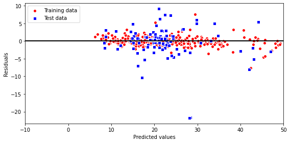

# 特徴量重要度を表示
model.feature_importances_

array([0.04127976, 0.00123856, 0.0075613 , 0.00087938, 0.02053643,
       0.40584637, 0.01357617, 0.03910201, 0.00384994, 0.0157941 ,
       0.0222856 , 0.00957269, 0.41847769])

# 特徴量重要性を計算
importances = model.feature_importances_

# 特徴量重要性を降順にソート
indices = np.argsort(importances)[::-1]

# 特徴量の名前を、ソートした順に並び替え
names = [boston.feature_names[i] for i in indices]

# プロットの作成
plt.figure(figsize=(8,4)) #プロットのサイズ指定
plt.title("Feature Importance")
plt.bar(range(X.shape[1]), importances[indices])
plt.xticks(range(X.shape[1]), names, rotation=90)

plt.show()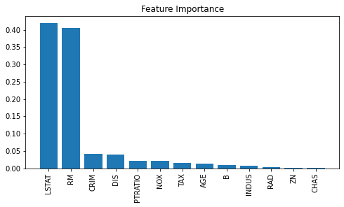

LSTAT：「低所得者人口の割合」
RM： 1戸当たりの「平均部屋数」
が住宅価格に影響を与える特徴量ということが分かる。

やってみて

特徴量重要性を計算抽出してグラフ化が、たったの数行で可能なのが驚き
競馬の馬柱データと着順に置き換えて分析したら楽しそうだと思った。